The world of artificial intelligence and machine learning has made remarkable strides in recent years. One fascinating application of machine learning is the recognition of handwritten digits, a task that may seem trivial to humans but is quite challenging for computers. In this blog, we will delve into the fascinating realm of Convolutional Neural Networks (CNNs) and explore how they enable machines to recognize handwritten digits with high accuracy.

Why Handwritten Digit Recognition?

Handwritten digit recognition has a wide range of applications, from reading postal codes on envelopes to interpreting bank checks, and even assisting in character recognition in various document management systems. The foundation of many modern machine learning and deep learning models, particularly in the field of computer vision, lies in the ability to recognize handwritten digits.

Introducing Convolutional Neural Networks (CNNs)

CNNs have revolutionized image processing and pattern recognition. They have become the go-to architecture for image-related tasks. Understanding how CNNs work and how they can be applied to problems like handwritten digit recognition is a fundamental step for any machine learning enthusiast.

In this blog, we will walk through the code that implements a CNN for recognizing handwritten digits using the MNIST dataset, a popular dataset in the field of machine learning. We'll break down the code into easily digestible sections, explain each part in detail, and help you grasp the underlying concepts.

Let's embark on this journey into the world of CNNs and see how they can distinguish between 0 and 9, just like we do!

In the next section, we'll delve into setting up the environment for this machine-learning task.

1. Setting up the Environment

Before we dive into the fascinating world of Convolutional Neural Networks (CNNs) and handwritten digit recognition, it's essential to ensure we have the right tools at our disposal. In this section, we'll introduce the key libraries and tools that make this code possible.

Meet the Libraries

In the code, we make extensive use of several libraries that are widely used in the machine learning and data science community:

• Matplotlib: This library is used for data visualization. It allows us to create various plots and charts to visualize the performance of our model, the data, and more.

• TensorFlow: TensorFlow is an open-source machine learning framework developed by Google. It's one of the most popular deep learning libraries and provides the tools necessary to build and train neural networks.

• Keras: Keras is a high-level neural network API, running on top of TensorFlow. It simplifies the process of building and training neural networks, making it easier for developers to create models.

• NumPy: NumPy is a fundamental package for scientific computing in Python. It provides support for arrays and matrices, making it an essential tool for numerical operations.

    import matplotlib as mpl
    import matplotlib.pyplot as plt
    import tensorflow as tf
    from tensorflow import keras
    import numpy as np
    import random
  

Facilitating Machine Learning and Data Visualization

These libraries work in harmony to help us build, train, and evaluate our CNN model. Matplotlib is used to visualize our data and model's performance, while TensorFlow and Keras are the backbone for creating and training our neural network. NumPy is used for array manipulations, especially during data preprocessing.

By using these libraries, we simplify the process of developing machine learning models and gain access to powerful tools for data analysis and visualization. Throughout this blog, we'll demonstrate how these libraries come together to create a seamless workflow for handwritten digit recognition.

In the next section, we'll explore how the code loads and preprocesses the data, a crucial step in any machine learning project.

2. Loading and Preprocessing the Data

In the world of machine learning, data is the foundation. For our handwritten digit recognition task, we need a reliable dataset to train and test our Convolutional Neural Network (CNN). In this section, we'll explore how the MNIST dataset is loaded and prepared for the task at hand.

Introducing the MNIST Dataset

The MNIST dataset is a collection of 28x28 pixel grayscale images of handwritten digits (0 through 9). It's a standard benchmark for image classification tasks and is widely used in the machine learning community. The dataset is divided into two main sets: one for training and another for testing. Each set contains images and corresponding labels.

mnist = tf.keras.datasets.mnist
(train_images, train_labels), (test_images, test_labels) = mnist.load_data()

In this code snippet, we import TensorFlow and Keras to help us manage the dataset. We use the load_data() function to fetch the MNIST dataset, splitting it into training and testing sets.

Data Normalization

Data preprocessing is a crucial step in machine learning. It involves preparing and cleaning the data to ensure that it's in the right format for training our model. In our case, we perform two essential preprocessing steps: normalization and one-hot encoding.

We normalize the pixel values of the images to a range of 0 to 1. This step ensures that the neural network's weights converge faster and the model is better equipped to learn the underlying patterns in the data. The following code accomplishes this:

train_images = train_images / 255.0
test_images = test_images / 255.0

Convolutional layers in our CNN expect a specific input shape. We reshape the images to have a single channel, which is essential for convolution operations:

train_images = train_images.reshape(-1, 28, 28, 1)
test_images = test_images.reshape(-1, 28, 28, 1)

The labels in the MNIST dataset are numerical values from 0 to 9. We convert these labels into a one-hot encoded format to make them compatible with our neural network. This means each label is transformed into a 10-element binary vector, with only one element being '1', indicating the digit's class. We achieve this using the following code:

train_labels = tf.keras.utils.to_categorical(train_labels, num_classes=10)
test_labels = tf.keras.utils.to_categorical(test_labels, num_classes=10)

By preprocessing the data in this manner, we ensure that it's ready to be fed into our CNN model for training.

In the next section, we will explore the architecture of our CNN model and how it learns to recognize handwritten digits.

3. Building the CNN Model

Now that we've loaded and preprocessed our data, it's time to create the heart of our handwritten digit recognition system - the Convolutional Neural Network (CNN). In this section, we'll explore the architecture of our CNN model and understand how it learns to recognize handwritten digits.

Understanding the CNN Architecture

A Convolutional Neural Network (CNN) is a type of neural network particularly well-suited for image recognition tasks. CNNs consist of layers designed to automatically and adaptively learn spatial hierarchies of features from the input images. The key components of a CNN include Convolutional layers, Pooling layers, and Fully Connected layers.

model = keras.models.Sequential()
model.add(keras.layers.Conv2D(32, (3, 3), activation='relu', input_shape=(28, 28, 1)))
model.add(keras.layers.MaxPooling2D((2, 2)))
model.add(keras.layers.Conv2D(64, (3, 3), activation='relu'))
model.add(keras.layers.MaxPooling2D((2, 2)))
model.add(keras.layers.Conv2D(64, (3, 3), activation='relu'))

• Sequential Model:

  We create a sequential model in Keras, which allows us to stack layers on top of each other, forming a linear pipeline.

• Convolutional Layers:

  Convolutional layers are the backbone of a CNN. They apply a set of learnable filters to the input data, which helps the model detect patterns and features within the images. In our code, we have three convolutional layers. Each layer consists of 32 or 64 filters, each with a 3x3 size. We use the 'ReLU' (Rectified Linear Unit) activation function to introduce non-linearity and enhance the model's ability to capture complex patterns.

• Pooling Layers:

  Pooling layers down-sample the spatial dimensions of the feature maps produced by the convolutional layers. This helps reduce the number of parameters and computations in the network. The 'MaxPooling2D' layers in our code use a 2x2 window to perform max pooling.

Next, let's look at how the model handles the fully connected layers:

model.add(keras.layers.Flatten())
model.add(keras.layers.Dense(64, activation='relu'))
model.add(keras.layers.Dense(10, activation='softmax'))

• Flatten Layer:

  Before we can feed the data into fully connected layers, we need to flatten the feature maps from the previous layers. The 'Flatten' layer reshapes the 2D feature maps into a 1D vector.

• Dense Layers:

  Dense layers, also known as fully connected layers, are traditional neural network layers. They learn patterns in the flattened feature vectors and make predictions. In our code, we have two dense layers. The last layer, with 10 units and a 'softmax' activation function, produces output probabilities for each digit class (0-9). The digit with the highest probability is the predicted digit.

Our CNN architecture is now ready to be compiled and trained to recognize handwritten digits. In the next section, we'll explore the process of compiling and training the model.

4. Compiling and Training the Model

Now that we've built our Convolutional Neural Network (CNN) architecture, it's time to get it ready for learning. In this section, we'll explore the compilation and training process, where our model will learn to recognize handwritten digits.

Model Compilation

Before we can train our model, we need to configure how it will learn. This is done during the compilation step. Key components of model compilation include the optimizer, loss function, and evaluation metrics.

model.compile(optimizer='adam', loss='categorical_crossentropy', metrics=['accuracy'])

• Optimizer:

  We use the 'Adam' optimizer, a popular choice for gradient-based optimization in deep learning. It adapts the learning rate during training, making it a suitable choice for many tasks.

• Loss Function:

  The 'categorical_crossentropy' loss function is used for multiclass classification problems, where each input belongs to one of several classes. It quantifies how well the predicted probabilities match the true labels.

• Metrics:

  During training, we want to keep track of the model's accuracy. 'accuracy' is a common metric used for classification tasks.

Training the Model

Training a neural network involves feeding it with the training data, allowing it to make predictions, and adjusting its internal parameters (weights) to minimize the loss. We specify several training parameters, including the number of training epochs and batch size.

history = model.fit(train_images, train_labels, epochs=5, batch_size=64, validation_data=(test_images, test_labels))

• Training Data:

  We use train_images and train_labels as the training data and corresponding labels.

• Epochs:

  An epoch represents one complete pass through the entire training dataset. In our code, we train for 5 epochs, which means the model will see the entire dataset 5 times during training.

• Batch Size:

  Training with the entire dataset at once can be computationally expensive. The 'batch_size' parameter specifies the number of samples that are processed before the model's internal parameters are updated. In our code, we use a batch size of 64.

• Validation Data:

  To monitor the model's performance during training, we use a separate dataset (test_images and test_labels) as validation data. This helps us ensure that the model generalizes well to unseen data.

Training a CNN may take some time depending on the complexity of the architecture and the size of the dataset. Once training is complete, we can evaluate the model's performance on the test data, which we'll cover in the next section.

In the following section, we'll evaluate the model to see how well it can recognize handwritten digits.

5. Evaluating the Model

Now that our Convolutional Neural Network (CNN) has been trained on the MNIST dataset, it's time to assess how well it can recognize handwritten digits. In this section, we'll evaluate the model's performance and calculate its accuracy on the test data.

Model Evaluation

To evaluate the model, we use the following code:

test_loss, test_acc = model.evaluate(test_images, test_labels)
print(f'Test accuracy: {test_acc * 100:.2f}%')

• model.evaluate(): This function takes the test data (test_images and test_labels) and computes the model's performance. It returns two values: test_loss (the loss on the test data) and test_acc (the accuracy on the test data).

• Printing Test Accuracy: We print the test accuracy as a percentage to assess how well the model performs on data it has never seen before. This metric helps us gauge the model's generalization ability.

The output of this code will show the test accuracy of the model, indicating how effectively it can recognize handwritten digits.

In the next section, we'll visualize predictions made by the model on randomly selected images from the test dataset, providing a more intuitive understanding of the model's performance.

6. Visualizing Predictions

To gain a practical understanding of how well our Convolutional Neural Network (CNN) is performing, we can visualize its predictions on randomly selected images from the test dataset. This section provides a more intuitive sense of the model's capabilities.

Randomly Selecting Test Images

We begin by randomly selecting four indices from the test dataset to showcase a few images. This code snippet helps us get a glimpse of the images the model will be making predictions on.

import random
# Randomly select 4 indices from the test data
random_indices = random.sample(range(len(test_images)), 4)

• random.sample(): This function randomly selects 4 indices from the range of indices corresponding to the test data. These indices are used to access the test images and labels.

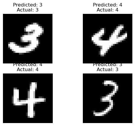
Iterating and Displaying Predictions

We then iterate through the selected indices and display the test images along with their predicted and actual labels. This code provides a visual representation of how well the model is recognizing handwritten digits.

for i, index in enumerate(random_indices):
    image = test_images[index].reshape(28, 28)  # Reshape back to 2D
    predicted_label = np.argmax(model.predict(np.expand_dims(test_images[index], axis=0))
    actual_label = np.argmax(test_labels[index])

    # Display the image
    plt.subplot(2, 2, i+1)
    plt.imshow(image, cmap='gray')
    plt.title(f"Predicted: {predicted_label}\nActual: {actual_label}")
    plt.axis('off')

plt.show()

• Reshaping Images:

  Before displaying the images, we reshape them back to their original 2D form. This is because the model expects input images in their original shape (28x28).

• Predicting and Comparing Labels:

  We use the model to predict the label for each selected image and compare it with the actual label from the test dataset. This allows us to showcase how well the model's predictions align with reality.

• Matplotlib for Visualization:

  We use Matplotlib, a popular Python library for data visualization, to display the images and labels in a user-friendly format.

By executing this code, you can visualize how well the model is performing on individual images, providing a tangible sense of its recognition capabilities.

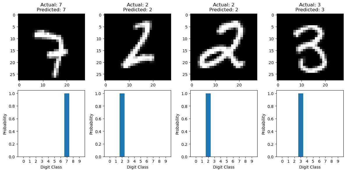
7. Visualizing Predictions with Probability Charts

In the previous section, we visualized the model's predictions on random test images. Now, let's take our visualization a step further by displaying probability charts for each digit class. This provides deeper insights into the model's decision-making process.

Iterating and Displaying Predictions with Probability Charts

We'll iterate through the selected indices and display the test images along with their predicted and actual labels. Additionally, we'll create probability charts showing the likelihood of each image belonging to a particular digit class.

plt.figure(figsize=(12, 6))

for i in range(4):
    plt.subplot(2, 4, i + 1)
    plt.imshow(selected_images[i].reshape(28, 28), cmap='gray')
    plt.title(f"Actual: {true_labels[i]}\nPredicted: {predicted_labels[i]}")

    # Plot the probability chart
    plt.subplot(2, 4, i + 5)
    plt.bar(range(10), model.predict(selected_images[i:i + 1])[0])
    plt.xticks(range(10), range(10))
    plt.xlabel("Digit Class")
    plt.ylabel("Probability")

plt.tight_layout()
plt.show()

• Image Display:

  We display the selected test images along with their actual and predicted labels, providing a clear visual representation of the model's recognition.

• Probability Charts:

  For each image, we create a bar chart showing the probability of the image belonging to each of the ten-digit classes (0-9). The predicted class will have the highest probability, and this chart illustrates the model's confidence in its prediction.

This visualization provides a deeper understanding of how the model makes predictions, including its level of certainty about each digit class. It's a powerful tool for interpreting the model's performance and decision-making.

Conclusion

In this journey through the world of Convolutional Neural Networks (CNNs) and handwritten digit recognition, we've explored the various aspects of building, training, and evaluating a model for this fascinating task. Here are the key takeaways from our exploration:

1. Convolutional Neural Networks (CNNs): CNNs are powerful tools for image recognition tasks. They are designed to automatically learn and detect features within images, making them ideal for recognizing handwritten digits.

2. MNIST Dataset: The MNIST dataset is a widely used benchmark for digit recognition. It contains thousands of 28x28 pixel grayscale images of handwritten digits, making it a perfect choice for training and testing machine learning models.

3. Data Preprocessing: Data preprocessing is essential for preparing the dataset for training. This includes normalizing pixel values, reshaping images, and one-hot encoding labels.

4. Model Architecture: We've seen how to build a CNN model with convolutional layers, pooling layers, and fully connected layers. These components work together to learn and recognize patterns within the data.

5. Model Training: Training a model involves configuring the optimizer, loss function, and evaluation metrics. We've used the 'Adam' optimizer and 'categorical_crossentropy' loss for our digit recognition task.

6. Model Evaluation: Evaluating the model's performance on the test data is crucial. Our code demonstrated how to calculate and print the test accuracy to assess how well the model generalizes to new data.

7. Visualizing Predictions: We've taken a closer look at how the model makes predictions by visualizing random test images and comparing predicted and actual labels. This helps us understand the model's recognition abilities.

8. Probability Charts: In the final stage, we enhanced our visualizations by displaying probability charts for each digit class, offering insights into the model's confidence in its predictions.

Convolutional Neural Networks have revolutionized the field of computer vision, enabling machines to perform tasks like handwritten digit recognition with remarkable accuracy. Their applications go far beyond recognizing digits, extending to various image recognition tasks, object detection, and more.

Finally, keep exploring, experimenting, and building, and you'll discover the boundless potential of machine learning in solving real-world problems. Till then adios!